1 What is Zero Filling? Why Do We Do It?
1.1 The Digital Resolution Problem
NMR data is acquired as a time domain signal - a series of voltage measurements from the receiver coil sampled at regular intervals. After Fourier transformation, this becomes our frequency domain spectrum. The key relationship governing digital resolution is:
Digital Resolution = Sampling Rate ÷ Total Number of Points
This creates a fundamental trade-off: to get better frequency resolution (more points), we need either faster sampling or longer acquisition times. However, there’s a practical limit - NMR signals decay exponentially, typically reaching the noise level within seconds.
1.2 The Zero-Filling Solution
Zero filling is the process of appending zeros to the end of the time domain data before Fourier transformation. This elegant technique provides more frequency points without the drawbacks of extended data collection:
1.2.1 Why Not Just Collect More Data?
Continuing data acquisition after signal decay has significant disadvantages:
- Increased noise: Every additional time point adds noise that spreads across all frequency points
- Longer experiment time: Exposes samples to degradation and increases costs
- Diminishing returns: No signal information gained after decay to noise level
1.2.2 The Zero-Filling Advantage
Appending zeros instead offers:
- No additional noise: Zeros contain no noise by definition
- Instant processing: No extra acquisition time required
- Better interpolation: More frequency points reveal peak shapes more accurately
- Improved quantification: Enhanced precision for peak integration and position measurement
Zero filling doesn’t create new information, but it does provide better digital representation of the continuous frequency spectrum that actually exists in your sample.
1.3 Demonstration: Comparing Three Acquisition Strategies
This demonstration illustrates the practical consequences of different data acquisition approaches using a realistic noisy FID signal at 15.15 Hz with exponential decay (R = 4 s⁻¹). We compare three scenarios that represent common experimental decisions:
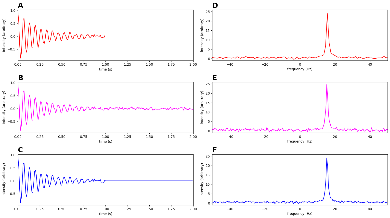
1.3.1 Time Domain Signals (Left Column):
Panel A - Optimal Acquisition: 1-second FID collected until signal decays to noise level
Panel B - Extended Acquisition: Same signal but acquisition continued for 2 seconds (collecting additional noise)
Panel C - Zero-Filled Strategy: The 1-second FID from Panel A zero-filled to match the 2-second length
1.3.2 Frequency Domain Results (Right Column):
Panel D - Standard Processing: Fourier transform of the 1-second FID (100 frequency points)
Panel E - Extended Processing: Fourier transform of the 2-second noisy acquisition (200 frequency points)
Panel F - Zero-Fill Processing: Fourier transform of the zero-filled FID (200 frequency points)
1.3.3 Key Experimental Parameters:
- Signal frequency: 15.15 Hz (chosen to fall on a digital frequency point)
- Decay rate: R = 4 s⁻¹ (realistic for many NMR experiments)
- Sampling rate: 100 Hz (bandwidth = ±50 Hz)
- Noise level: Added to simulate real experimental conditions
This comparison will reveal why zero-filling (Panel F) provides superior results compared to simply extending acquisition time (Panel E), while maintaining the same digital resolution as the extended acquisition.
In the data above, we can see that (B) takes twice as long to acquire as (A), and the second half of (B) is mainly composed of noise. If that sounds like that’s a bad thing, you would be right. Again, if our signal has decayed to the noise level, there is no point in continuing to collect data. Instead, we remove the noise if we add zeros to the data for this period, like in (C). What effect does this have on our Fourier Transforms in (D), (E), and (F)?
1.4 Effect of Zero-filling on Resolution and Noise
This comparison demonstrates two critical benefits of zero-filling: reduced noise and improved digital resolution. The panels below compare three acquisition strategies using the same underlying signal:
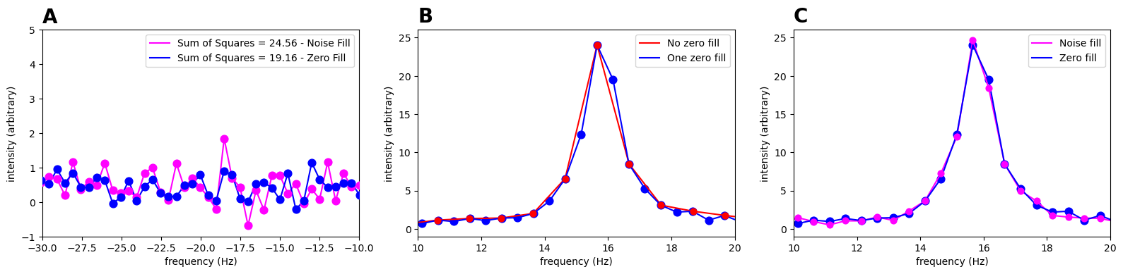
Panel A - Noise Comparison: Examines baseline noise levels away from the peak region. The magenta spectrum shows data collected for 2 seconds (continuing acquisition after signal decay), while the blue spectrum shows the same signal truncated at 1 second and zero-filled to 2 seconds. The sum of squares values quantify the noise difference - zero-filling significantly reduces baseline noise while requiring less acquisition time.
Panel B - Digital Resolution: Overlays the original spectrum (red, 100 points) with its zero-filled version (blue, 200 points). Notice that zero-filling doubles the number of frequency points without changing the original data - every red point has a corresponding blue point at exactly the same frequency and intensity. This demonstrates that zero-filling is true interpolation, not data modification.
Panel C - Direct Comparison: Shows the same frequency range for both acquisition strategies. The magenta points (noise-filled) show greater scatter around the true peak shape compared to the blue points (zero-filled). While longer acquisition provides more actual data, the benefits are negated by the added noise after signal decay.
Key Insight: Zero-filling provides the benefits of longer acquisition time (more frequency points) without the penalty of collecting noise, making it an essential processing step for high-quality NMR spectra.
1.5 Why We Push Zero-Filling Past One Zero Fill
While a single zero-fill doubles our frequency points and reveals basic peak shape information, there are compelling reasons to apply more aggressive zero-filling. The critical question is: How precisely can we determine the exact frequency (or chemical shift) of a peak?
1.5.1 The Digital Precision Challenge
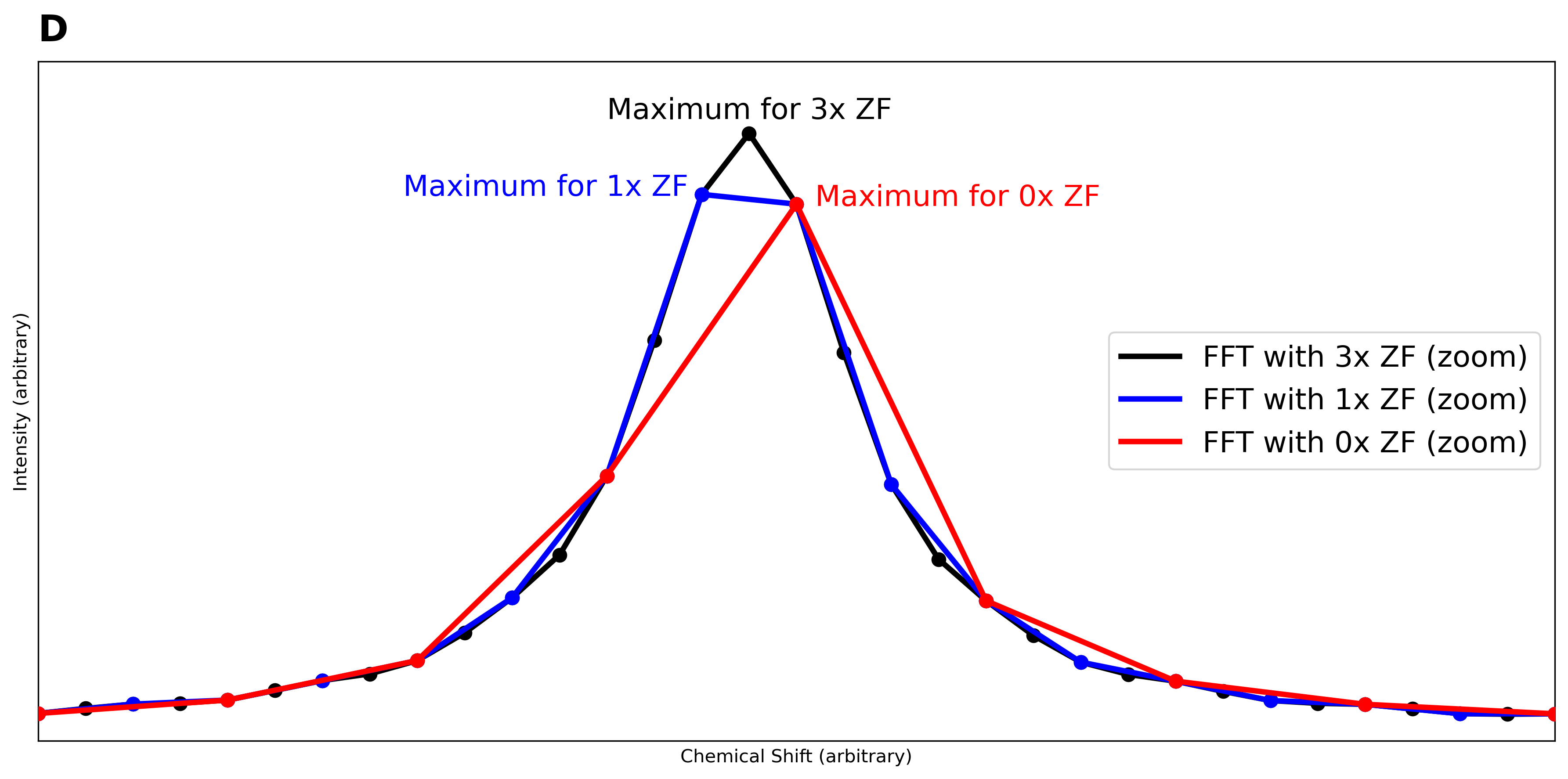
In this demonstration, we use a signal at 24.74 Hz - deliberately chosen to fall between natural digital frequency points - to illustrate how limited digital resolution can miss the true peak center. With insufficient frequency sampling, peak maxima may appear at incorrect positions, leading to systematic errors in quantitative analysis.
1.5.2 Benefits of Extended Zero-Filling
The more zero-filling we apply, the denser our frequency grid becomes, providing:
- Enhanced peak localization - More frequency points around the peak enable precise identification of the true maximum
- Improved quantitative accuracy - Peak integration and intensity measurements become significantly more reliable
- Better spectral interpolation - Peak shapes are more accurately represented with higher point density
- Reduced systematic errors - Critical for applications like relaxation measurements and kinetic studies
1.5.3 Panel-by-Panel Analysis
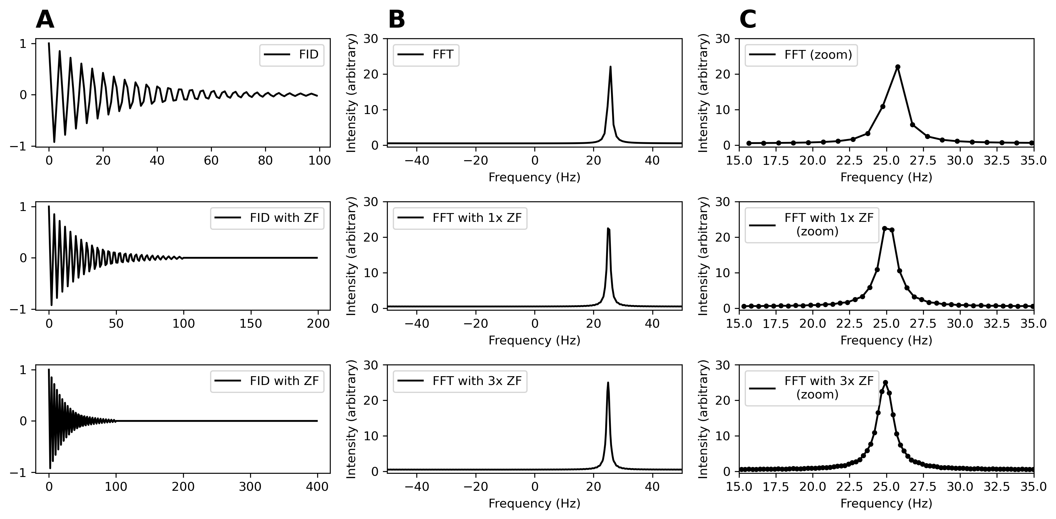
The comparison below demonstrates progressive zero-filling effects using the same 24.74 Hz signal:
Column A - Time Domain: Shows how zero-filling modifies the FID by appending zeros, with increasing numbers of added points from top to bottom (0x, 1x, 3x zero-fill).
Column B - Full Spectra: Reveals how additional zero-filling increases the number of frequency points across the entire spectrum, with identical peak positions but progressively better digital sampling.
Column C - Peak Zoom: Focuses on the 15-35 Hz region to clearly demonstrate how increased zero-filling provides finer frequency resolution around the peak, making peak shape and position more apparent.
Panel D - Direct Overlay: Superimposes all three zero-filling levels on the same frequency scale, dramatically illustrating how additional zero-filling reveals progressively better peak definition and more accurate peak position determination - essential capabilities for quantitative NMR analysis.